I've been (ab)using LLMs for quite a while now. When I saw the inflection point in OpenAI's models starting from GPT, I knew it was time to quit my job and try building as a solo developer. @bountycaster effectively was the birthchild of AI's progress: I was prompting models to speed up building (no Claude Code at the time), my AI agent was built on top of OpenAI APIs and Farcaster, I was using Deep Research to think about the product.

As much as I understand the application layer of LLMs (tool calling, context, embeddings, etc) - I didn't know how the thing actually worked, and that felt very limiting.

So I decided to build a tiny LLM from scratch. Not to become an ML researcher, but because I believe that if you build something yourself, even a toy version, you start to see the shape of the real thing. There is also a competitive advantage of being able to read papers, compare architectures, and make better decisions - even if I keep on building at the application layer.

Learning bottoms up

A few reasons to build bottom-up:

• Transformer architecture isn't insanely complex, understanding core components in isolation makes it easier to digest
• Papers become more readable, since they assume you know what a Head, Block, embedding, norm is. You learn to see these components as lego pieces and appreciate how researchers plug and play them in different parts of the network.

Using Claude as my Sherpa

I've been slowly mastering the art of "learning with LLMs". You can put Claude Code into learning mode config -> output and ask it questions guiding you through the process. You write 100% of the code (it's good for learning) and the agent corrects you and builds on top of your solution.

I strongly believe this is a very underrated way of using LLMs: you should have the agency to understand what tasks can be fully delegated, and which ones should be learned - the best things to learn are the ones with compounding payoff. In this particular scenario, using LLMs to learn LLMs will compound.

A small rundown

There is no substitute to actually going through this video that was golden (thank you @karpathy) which took a few days if you want to really dig deep and understand the core components. Below is a rundown of what I learned, this article is very selfish since I am using it as a way to solidify information.

Notation

A few dimensions that come up everywhere. I'll use these consistently:

• T — sequence length (number of tokens in the input)
• C — embedding dimension (size of each token's vector representation)
• h — head size per attention head (C / number of heads)
• V — vocabulary size (total tokens the tokenizer knows)

Tokenizers

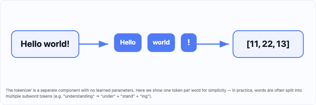
This is probably the easiest part to grasp as a software engineer. A tokenizer is essentially a pure function that maps a string to a list of integers.

encode("Hello world!") -> [11, 22, 13, 24, 1]
decode([11, 22, 13, 24, 1]) -> "Hello world!"

The tokenizer is the only part of the pipeline that is completely separate from the neural network. It has no learned parameters. It's just a lookup table agreed upon before training/inference starts.

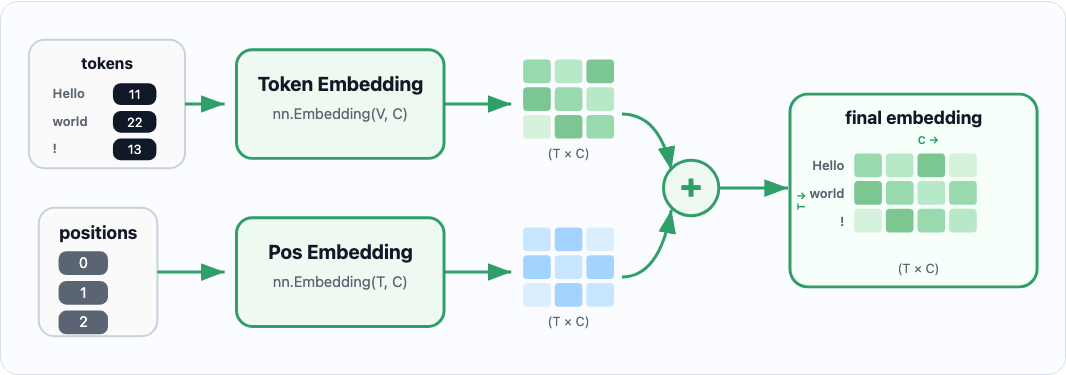
Embeddings: Giving Tokens a Location in Space

Before any attention happens, raw token indices (integers) get turned into dense vectors. There are two embedding tables:

• Token embeddings: map each token in the vocabulary to a vector. The model learns what each token means in terms of a C-dimensional vector. This is seen as nn.Embedding(vocab_size, embedding_size)
• Positional embeddings: map each position in the context window to a vector. This "marks" each embedding with information regarding the position.

embeddings = token_embeddings(X) + positional_embeddings(X)

^ the above generates a T x C matrix, where T is the token sequence, and C is the embedding dimension.

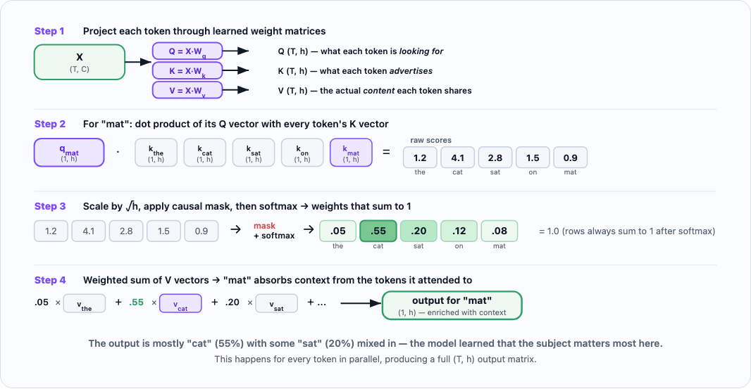
The attention head

This is the core of the transformer. The goal is to train 1 or more heads to pay attention to past areas of the context window. The question attention answers is: "for each token, which previous tokens are most relevant?"

How does this work: each head contains a K, V, Q matrix - initiated with random weights, that trains to absorb specific meaning from the words in the context. With one particular trick, we only allow characters at position t to "connect" with characters <= t. This allows for causal prediction: the model only ever uses past context to predict the next token, never future tokens.

X # (T, C) — T tokens, each with a C-dimensional embedding

# Project to Q, K, V — each becomes (T, h)
q = self.Q(X) # what each token is looking for
k = self.K(X) # what each token is advertising
v = self.V(X) # the features each token will share

# Compute attention scores: (T, h) @ (h, T) → (T, T)
weights = q @ k.transpose() # Omitting head size scaling here for simplicity

# Mask out future tokens: set upper triangle to -inf so softmax → 0
# weights[i][j] = -inf where j > i (token i cannot see token j)
weights = softmax(weights, dim=-1)

# Weighted sum of values → (T, h)
out = weights @ v

As someone who learns a lot visually, I asked Claude to generate some interactive examples of the attention process so I could fully understand them. I deployed them here (thank you @here_now).

Here's what the full attention computation looks like step by step, tracing how "mat" decides which earlier tokens matter:

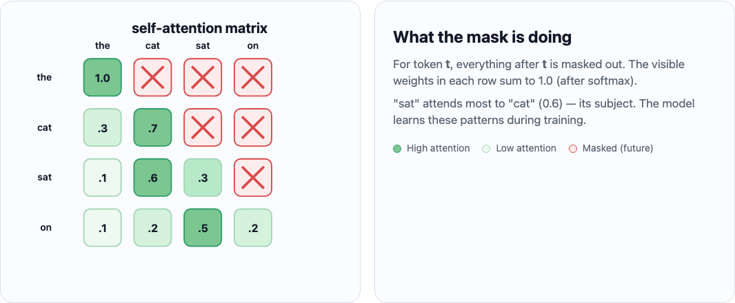
The causal mask ensures each token can only attend to tokens that came before it. Here's what the resulting weight matrix looks like — notice how each row sums to 1.0 and future tokens are blocked:

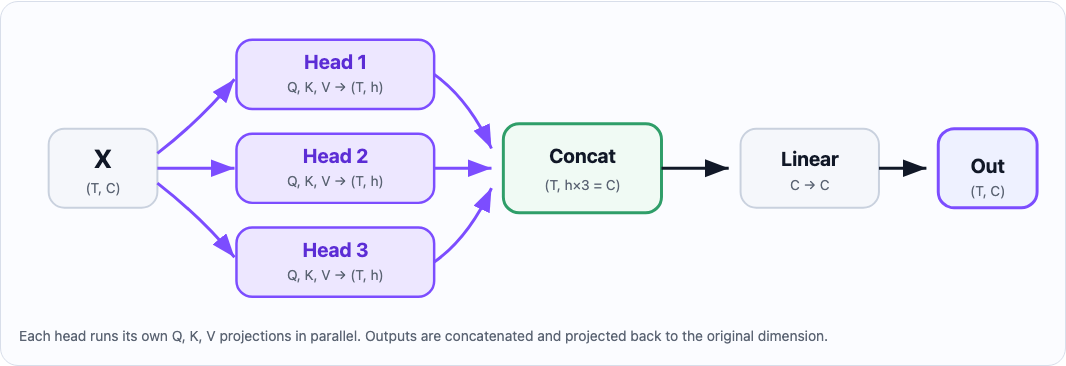
Adding multiple heads for attention

The attention mechanism can also be empowered by training multiple heads instead of simply one, and then subsequently recombining them. Each head learns to attend to a different type of relationship in the sequence, you don't tell them what to specialize in; it emerges from training.

The core requirement is that head_size = embedding_dim / num_heads. You pick the number of heads, and head size follows.

The implementation is straightforward: run N heads in parallel on the same input, then concatenate their outputs and project back via a single linear layer. The linear layer is used to ensure the final representation picks the most useful bits of each block.

# head(X) will return T x head_size. Concatenating all heads together will lead to embedding_dim.
out = nn.concat([head(X) for head in heads])

out = linear_layer(out) # This is simply a `nn.Linear(embedding_dim, embedding_dim)`

# out is now a T x embedding_dim

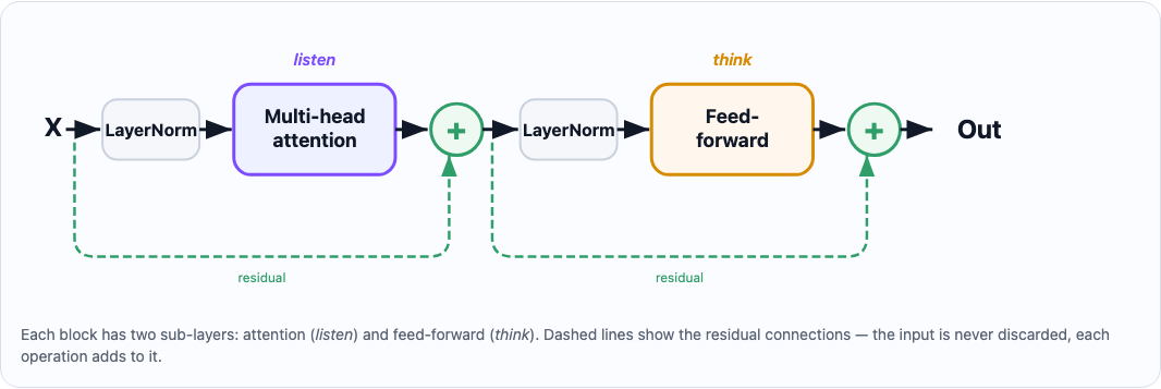
Putting Everything in a Block

Now that we have our building blocks, let's assemble them into a Block class. Blocks run sequentially: the more blocks, the more complexity our network can bear, but also the more layers of abstraction it can learn. This is the transformer equivalent of "how many hidden layers?" in a classic neural network: deeper means harder to train, but also richer representations.

Each block contains:

• Multi-head attention: lets the model figure out which tokens to pay attention to
• Feed-forward network (with ReLU activation): processes what attention found and draws conclusions
• LayerNorm before each sub-layer: stabilizes training

The block is also called a residual block because the input X is never discarded — each operation adds to it rather than replacing it.

X # (T, dim_embeddings)
X += multi_head_attention(layernorm(X))
X += feed_forward(layernorm(X))
return X

A useful analogy (thank you Claude): attention is like reading the room, figuring out who said what and who deserves your focus. Feed-forward is like thinking it over — processing what you just heard and forming conclusion. Every block does one round of listen, then think. Stack enough blocks and you get something that can reason.

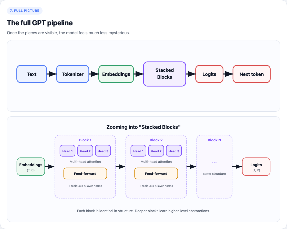
Putting it all together

Once you have the lego pieces above, putting it together is plumbing. Here is the recipe:

For any token input X such as [11, 22, 13, 24, 1], you do the following:

X = [11, 22, 13, 24, 1] # sequence of length T

# Fetch embeddings for each token
X = embeddings(X) # Now this is (T, C) -> where C is the embedding dimension

# run blocks one at a time (each block contains multi-head attn + feed-forward)
for block in blocks:
    X = block(X)

# Final output layer: layernorm + linear layer back to n_vocab
X = embeddings_to_vocab(ln(X))
return X # This can now be decoded using the token decoder

What's next

Three concepts I want to understand next, each mapping directly onto a part of the architecture above:

• RoPE: replaces the positional embedding table. Instead of adding position vectors to token embeddings, it rotates Q and K inside each head based on relative position. Most modern LLMs use this.
• Mixture of Experts: instead of having one single feed-forward layer after multi-head attention, you have a router that picks a subset for each token.
• LoRA: a fine-tuning technique.

Code I wrote for this tutorial

Here's the full implementation I wrote while learning this way — Claude as the sherpa, me writing every line: view on GitHub Gist.

AI usage

The first draft of the article was written by me, I used Claude to tidy up, shorten, and clarify areas that needed some touch up. 100% of pictures were made via Opus 4.6 (I was opinionated in tweaking the design and what to show).